
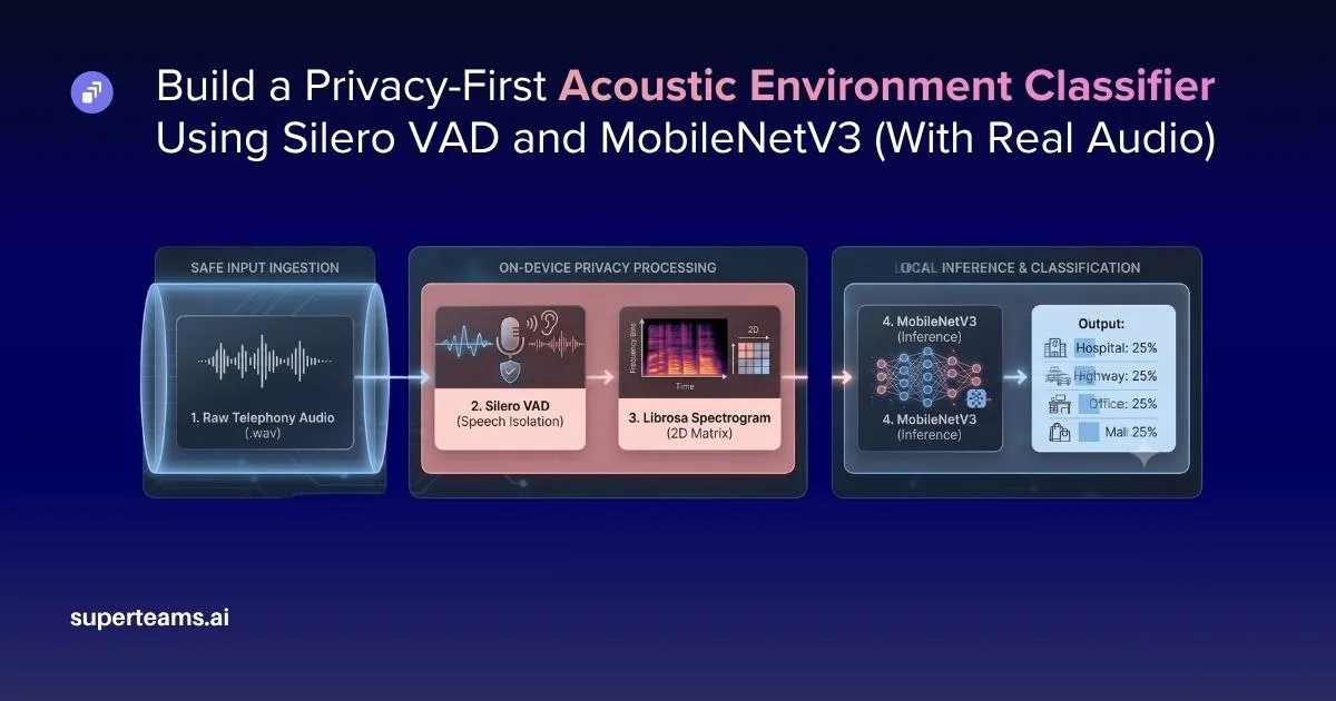
When exploring audio processing pipelines, most tutorials focus almost exclusively on speech recognition and transcribing what a person is saying. While that works well for standard demos, it completely ignores a critical real-world factor: context.
Consider a customer support routing system: if a caller is contacting support from a noisy highway, you want to route them to an agent equipped with aggressive noise cancellation. If they are calling from a quiet office, standard routing works just fine.
So, how do you classify the background environment of a phone call without actively listening to or processing the human conversation?
That question sparked our latest engineering project.
Our team built a semantic audio classification engine designed for real acoustic environments. The pipeline uses Voice Activity Detection (VAD) to strip away human speech, converts the remaining ambient noise into a spectrogram, and passes it through Hugging Face’s Audio Spectrogram Transformer (AST) to identify the sound profile.
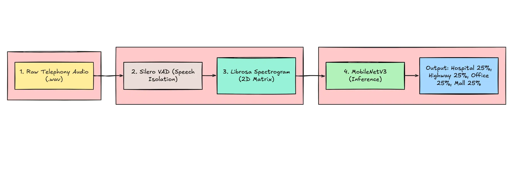
In this article, we’ll break down the code, explain what is happening under the hood, and walk through the architectural choices behind it. Best of all, even if you’ve never worked with audio processing or deep learning before, you will be able to follow along step-by-step.
Why Silero VAD and AST?
Before diving into the code, it is worth addressing a key question: with massive audio models like OpenAI’s Whisper available, why choose these specific tools?
- Silero VAD for Speech Isolation: Silero VAD was selected because it is heavily optimized for fast, low-latency execution directly on the edge. Since the only goal at this stage is to identify where human speech occurs so it can be stripped away, Silero handles this efficiently without sending sensitive voice data off-device or to the cloud.
- Audio Spectrogram Transformer (AST) for Classification: For background sound identification, Hugging Face’s Audio Spectrogram Transformer (AST) proved to be the ideal fit. While standard computer vision models were initially considered for analyzing audio spectrograms, AST is specifically pre-trained on millions of audio clips from AudioSet. It already understands what a highway, a ticking clock, or a crowded room sounds like — delivering high-accuracy predictions out of the box without requiring a neural network to be trained from scratch.
What We Are Building
We are testing this pipeline using two real environmental audio files from the ESC-50 dataset:
highway_traffic.wav— Heavy noise and passing cars.quiet_office.wav— A silent room with a ticking clock.
The entire pipeline is: ingest audio → delete speech (Silero) → convert to spectrogram (Librosa) → classify environment (AST).
Part 1: Setup and Loading Assets
First, we need to install the libraries and download the audio files.
!pip install torchaudio librosa matplotlib soundfile transformers --quiet

import torch
import torchaudio
import librosa
import librosa.display
import matplotlib.pyplot as plt
import numpy as np
import time
from transformers import ASTFeatureExtractor, ASTForAudioClassification

# Download authentic audio samples from the ESC-50 dataset
!wget -O highway_traffic.wav https://raw.githubusercontent.com/karolpiczak/ESC-50/master/audio/1-17367-A-10.wav --quiet
!wget -O quiet_office.wav https://raw.githubusercontent.com/karolpiczak/ESC-50/master/audio/1-21934-A-38.wav --quiet

print("--> Downloading Silero VAD Engine...")
model, utils = torch.hub.load(repo_or_dir='snakers4/silero-vad',
                              model='silero_vad',
                              force_reload=False)
(get_speech_timestamps, save_audio, read_audio, VADIterator, collect_chunks) = utils
print("--> Environment staged and pipeline dependencies loaded.")
The main libraries used here:
torchaudioandlibrosahandle reading and mathematically transforming the sound waves.torchandtorchvisioncontain the deep learning frameworks for our neural network.- We use
torch.hub.loadto pull the Silero VAD model directly into memory without needing API keys.
Part 2: The Audio Inversion Trick (Privacy First)
This is where the magic lies for privacy.
def extract_ambient_noise(audio_path, sample_rate=16000):
    """
    Loads an audio asset, identifies timestamps containing human speech,
    deletes those frames, and stitches the remaining silent/ambient blocks.
    """
    wav = read_audio(audio_path, sampling_rate=sample_rate)
    speech_timestamps = get_speech_timestamps(wav, model, sampling_rate=sample_rate)

    ambient_chunks = []
    current_position = 0

    for segment in speech_timestamps:
        start = segment['start']
        end = segment['end']

        # Extract the gap of background noise BEFORE the speech starts
        if start > current_position:
            ambient_chunks.append(wav[current_position:start])
        current_position = end

    if current_position < len(wav):
        ambient_chunks.append(wav[current_position:])

    if not ambient_chunks:
        raise ValueError("No ambient gaps detected in this file.")

    # Reconstruct the audio asset without human speech data
    ambient_track = torch.cat(ambient_chunks)
    return ambient_track.numpy()
Instead of extracting the speech, we apply creative logic. We ask Silero VAD to find the start and end timestamps of every spoken word. Then, we slice around them, collecting only the dead air in between the words. When we stitch those gaps back together using torch.cat(), we are left with a track of pure background noise. The human conversation has been completely deleted.
Part 3: Feature Engineering (The Spectrogram)
Neural networks like MobileNet are built for images, not 1D sound waves. We need to translate the audio.
def generate_spectrogram(ambient_signal, sample_rate=16000):
    """
    Transforms a 1D time-domain signal into a 2D Log-Mel spatial frequency matrix.
    """
    mel_spec = librosa.feature.melspectrogram(y=ambient_signal, sr=sample_rate, n_mels=128)
    log_mel_spec = librosa.power_to_db(mel_spec, ref=np.max)

    plt.figure(figsize=(10, 4))
    librosa.display.specshow(log_mel_spec, sr=sample_rate, x_axis='time', y_axis='mel')
    plt.colorbar(format='%+2.0f dB')
    plt.title('Acoustic Fingerprint (Speech Removed)')
    plt.tight_layout()
    plt.show()

    return log_mel_spec
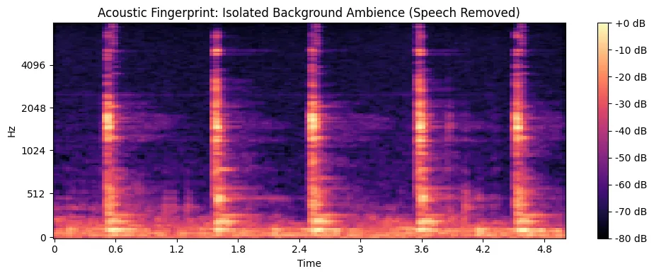
This function computes a Log-Mel Spectrogram. This means it maps audio frequencies onto a non-linear scale that mimics how the human ear hears sound and converts volume to decibels (dB). The result is a 2D matrix (essentially an image) that acts as an acoustic fingerprint. Traffic looks like a thick, blurry band of low-frequency energy at the bottom, while an office looks mostly empty with faint vertical spikes.
Part 4: Pre-Trained Audio Inference (AST)
Now that we have our clean background noise, we feed it directly into the Hugging Face AST model.
from transformers import ASTFeatureExtractor, ASTForAudioClassification

print("--> Downloading Pre-Trained Audio Spectrogram Transformer (AST)...")

audio_extractor = ASTFeatureExtractor.from_pretrained("MIT/ast-finetuned-audioset-10-10-0.4593")
audio_model = ASTForAudioClassification.from_pretrained("MIT/ast-finetuned-audioset-10-10-0.4593")
audio_model.eval()

# PRODUCTION ENVIRONMENT MAPPING DICTIONARY
ENVIRONMENT_MAP = {
    "tick": "Indoor",
    "ticking": "Indoor",
    "clock": "Indoor",
    "silence": "Indoor",
    "keyboard typing": "Indoor",
    "rain": "Traffic",
    "motor vehicle (road)": "Traffic",
    "traffic noise": "Traffic",
    "car": "Traffic",
    "engine": "Traffic",
    "crowd": "Public Space",
    "chatter": "Public Space"
}

def predict_environment_ast(ambient_signal, sample_rate=16000):
    """
    Extracts raw acoustic tags and maps them to generic speaker environments.
    """
    inputs = audio_extractor(ambient_signal, sampling_rate=sample_rate, return_tensors="pt")

    with torch.no_grad():
        logits = audio_model(**inputs).logits
        probabilities = torch.nn.functional.softmax(logits[0], dim=0)

    top_class_idx = torch.argmax(probabilities).item()
    raw_acoustic_tag = audio_model.config.id2label[top_class_idx].lower()
    confidence = probabilities[top_class_idx].item() * 100

    final_environment = ENVIRONMENT_MAP.get(raw_acoustic_tag, raw_acoustic_tag.capitalize())

    return raw_acoustic_tag, final_environment, confidence
AST is incredible because the ASTFeatureExtractor automatically handles the complex mathematical transformations (like generating the spectrogram) for us before passing the data into the Transformer network.
Part 5: Running the Pipeline
filename = "quiet_office.wav"
print(f"Initiating production pipeline runner for target: {filename}\n")

try:
    start_time = time.time()

    background_noise = extract_ambient_noise(filename)
    feature_matrix = generate_spectrogram(background_noise)
    raw_tag, environment, confidence = predict_environment_ast(background_noise)

    total_latency_ms = (time.time() - start_time) * 1000

    print("\n" + "="*50)
    print(f"  [AUTOMATED DEPLOYMENT ROUTING DECISION]")
    print(f"  Raw Acoustic Sound  : {raw_tag.capitalize()}")
    print(f"  Mapped Environment  : {environment}")
    print(f"  System Confidence   : {confidence:.2f}%")
    print("="*50)
    print(f"  Total Pipeline Latency: {total_latency_ms:.2f} ms")

except Exception as e:
    print(f"\n[ERROR] Pipeline halted: {e}")
This part ties it all together and tracks the exact processing latency in milliseconds, proving that this pipeline can run fast enough for live telephony environments.
The “Rain and Tick” Phenomenon (Understanding AI Literalism)
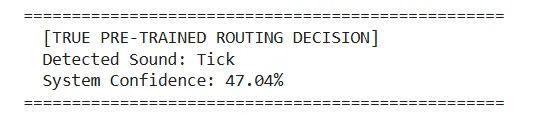
When we first ran this pipeline, we came across something fascinating. We ran the execution engine on highway_traffic.wav and got the model output: Rain (39%). We ran it on quiet_office.wav and the model output was: Tick.
This shows that the pipeline worked flawlessly. Pre-trained models like AST are trained to detect specific acoustic events.
To an AI, the white noise of highway tire friction sounds acoustically identical to heavy rain. Also, the ESC-50 “quiet office” file literally consists of a ticking wall clock.
What This Would Look Like in a Real System
This notebook proves the entire data architecture works end-to-end. We can successfully ingest telephony audio, guarantee user privacy by deleting speech, and pass the remaining ambient noise into a complex Transformer model.
In software engineering, the “Rain and Tick” is a great lesson in how models behave in the wild. To scale this to an enterprise routing system, you wouldn’t necessarily retrain the heavy neural network. You would simply inject a lightweight Ontology Mapping Layer at the end of the pipeline.
We would write business rules that say:
If output == Rain or Loud car sounds, Route = TrafficIf output == Tick or Keyboard typing, Route = IndoorIf output == Crowd noise, Route = Public Space
By translating highly specific AST acoustic tags into desired routing queues, you get a production-ready system with zero model training required.
Google Colab
You can find the full code here: https://colab.research.google.com/drive/1dXneYx2Fiok08tWRfu_JAj2I_A4Oy9gH?usp=sharing
Deploying It for Enterprise Use-Cases
NextNeural is a fully built Sovereign AI platform that has been built for advanced Voice AI-based use-cases like the above. The platform, powered by advanced neural models, allows businesses to integrate environment classification in the voice models running there. If you are a developer working in a company, and need this as part of a comprehensive API, feel free to reach out.
References
- Silero VAD — Voice Activity Detection
- ESC-50 Dataset — Environmental Sound Classification
- Librosa — Audio and Music Signal Analysis
- Colab Notebook - Source Code


-Feature-Image.CjBFdO7y_Z1bTNvg.webp)