Have you ever been on a call where the other person sounds like they’re standing next to a high-speed fan or a busy street? That background noise isn’t just annoying, it actively makes speech harder to understand. For machines (speech recognition systems, voice assistants), it’s even worse. A noisy signal can completely throw off a model that was trained on clean audio.
Speech enhancement is the process of pulling clean speech out of a noisy recording. It shows up everywhere:
- Voice assistants (Alexa, Google Assistant) need clean input to understand commands
- Telecom systems use it so calls don’t sound like static
- Hearing aids apply it in real time to help users focus on voices
- Video conferencing (Zoom, Meet) uses it so background noise doesn’t bleed through
- Automatic speech recognition (ASR) pipelines rely on it as a preprocessing step
The challenge is that noise comes in many forms — steady hum, sudden impulse sounds, traffic, keyboard clicks — and no single method handles all of them equally well.
What Is Speech Enhancement, Really?
At its core, speech enhancement tries to answer: given a signal that is speech + noise, how do I get back just the speech?
There are two main approaches:
Traditional Signal Processing Methods: These use mathematical rules about how signals behave. They don’t “learn” from data; they apply fixed formulas. Think of them as filters built on assumptions (e.g., noise is stationary, or noise is present only where speech is absent). They’re fast and lightweight but can struggle with unpredictable noise.
Deep Learning Methods: These train a neural network on thousands of noisy/clean pairs. The network figures out on its own how to separate speech from noise. They generalize better to real-world conditions but need more compute power. SpeechBrain falls in this category.
Both approaches have their place. The right choice depends on your use case: are you on a low-power embedded device, or do you have a GPU-backed server?
Methodology: How Each Model Works
Spectral Gating
Spectral gating works in the frequency domain. It first estimates what the noise “looks like” by sampling a quiet portion of the audio (or using a statistical estimate). Then, for each frequency bin, if the signal energy is below a threshold (the “gate”), it gets suppressed. Only the parts loud enough to be speech pass through.
In this experiment, the Python library noisereduce was used, which implements an improved version of spectral gating.
Spectral subtraction is a simple and widely used noise suppression technique that estimates the noise spectrum from a noise-only segment of the audio and subtracts it from the noisy speech spectrum. Since it does not require any training data or complex models, it is easy to implement and works effectively in environments with relatively constant background noise such as fan sounds, air conditioners, or engine hum. The method operates in the frequency domain using the Short-Time Fourier Transform (STFT), making it computationally efficient for many real-time applications.
However, spectral subtraction has certain limitations. The subtraction process can introduce a residual artifact known as musical noise, which sounds like random tonal fluctuations in the background. Its performance also degrades when dealing with non-stationary noise sources such as keyboard clicks, traffic sounds, or sudden disturbances because the noise estimate may no longer accurately represent the changing environment. Despite these drawbacks, the computational complexity remains relatively low to moderate, as it mainly involves forward and inverse STFT operations without requiring any deep learning models or extensive training procedures.
# Load audio
audio, sr = librosa.load(
    INPUT_FILE,
    sr=16000
)

# Audio duration
duration = len(audio) / sr

# Start timer
start = time.perf_counter()

# Spectral Gating
reduced = nr.reduce_noise(
    y=audio,
    sr=sr
)

# End timer
end = time.perf_counter()

# Calculate metrics
latency = end - start
rtf = latency / duration

# Save output
sf.write(
    OUTPUT_FILE,
    reduced,
    sr
)
Wiener Filter
The Wiener filter is a classic signal processing technique. It estimates the optimal linear filter that minimizes the mean squared error between the cleaned signal and the true clean signal. In practice, it uses the estimated signal-to-noise ratio at each frequency to decide how much to suppress each frequency component.
H(f) = S_speech(f) / (S_speech(f) + S_noise(f))Where H(f) is the filter gain, S_speech is the estimated speech power, and S_noise is the noise power. scipy.signal.wiener was used here — a simple, fast implementation.
- Advantages: Theoretically optimal under Gaussian noise assumptions, very fast, no artifacts.
- Limitations: Assumes stationary noise and Gaussian statistics — real-world noise often violates both. Output can sound slightly “muffled.”
- Computational complexity: Very low. A single-pass filter operation — among the fastest methods tested.
audio, sr = librosa.load(INPUT_FILE, sr=16000)
start = time.perf_counter()
enhanced = wiener(audio)
end = time.perf_counter()
latency = end - start
wiener_output = "wiener_demo.wav"
sf.write(wiener_output, enhanced, sr)
duration = len(audio) / sr
rtf = latency / duration
Median Filter
The median filter is a non-linear smoothing filter. It slides a small window along the signal and replaces each sample with the median value of its neighbors. This is especially good at removing short-duration spike-like noise (impulse noise) without blurring the signal much.
enhanced = medfilt(audio, kernel_size=5)A kernel size of 5 means each output sample is the median of itself and its 4 neighbors.
- Advantages: Extremely simple and fast. Very good at removing clicks, pops, and short impulse noise.
- Limitations: It is not designed for broadband or stationary noise. It can distort speech if the noise has similar duration to phonemes. It is also not effective against sustained background noise.
- Computational complexity: Very low. O(n log k) where k is the kernel size — practically instant.
audio, sr = librosa.load(INPUT_FILE, sr=16000)
start = time.perf_counter()
enhanced = medfilt(audio, kernel_size=5)
end = time.perf_counter()
latency = end - start
median_output = "median_demo.wav"
sf.write(median_output, enhanced, sr)
duration = len(audio) / sr
rtf = latency / duration
Spectral Subtraction
How it works: This is one of the oldest and most intuitive methods. The idea is: estimate the average noise spectrum from a “noise-only” portion of the signal (usually the first few frames), then subtract that estimate from every frame.
|S_clean(f)| = max(|S_noisy(f)| - |S_noise_est(f)|, 0)The max(..., 0) part ensures we don’t get negative magnitudes (half-wave rectification). The phase from the original noisy signal is kept, and inverse STFT reconstructs the waveform.
In the code:
noise_est = np.mean(magnitude[:, :10], axis=1, keepdims=True)
magnitude_clean = np.maximum(magnitude - noise_est, 0)
The first 10 frames are used as the noise estimate.
- Advantages: Simple, interpretable, and quick — gives reasonably clean output when noise is stationary.
- Limitations: The subtraction can leave residual noise artifacts (musical noise), similar to spectral gating. This method is very sensitive to the accuracy of the noise estimate: if the first 10 frames contain speech, the results degrade.
- Computational complexity: Low. Dominated by STFT/iSTFT operations.
audio, sr = librosa.load(INPUT_FILE, sr=16000)
start = time.perf_counter()
D = librosa.stft(audio)
magnitude = np.abs(D)
phase = np.angle(D)
noise_est = np.mean(magnitude[:, :10], axis=1, keepdims=True)
magnitude_clean = np.maximum(magnitude - noise_est, 0)
reconstructed = librosa.istft(magnitude_clean * np.exp(1j * phase))
end = time.perf_counter()
latency = end - start
sf.write(spectral_sub_output, reconstructed, sr)
duration = len(audio) / sr
rtf = latency / duration
SpeechBrain (Deep Learning)
SpeechBrain uses a trained neural network (mtl-mimic-voicebank) that has seen thousands of noisy/clean pairs. The model uses spectral masking; it predicts a mask for each time-frequency bin that represents how much of that bin belongs to speech. Multiplying the noisy spectrogram by this mask gives the enhanced speech.
Unlike the traditional methods above, this model doesn’t use a hand-crafted rule. It has learned what speech looks like across a wide range of noise conditions.
enhancer = SpectralMaskEnhancement.from_hparams(
    source="speechbrain/mtl-mimic-voicebank"
)
enhancer.enhance_file(INPUT_FILE, "speechbrain_demo.wav")- Advantages: Best overall quality and noise suppression. It handles non-stationary, complex noise and generalizes across noise types because of training diversity.
- Limitations: Needs a pretrained model (download required) and is the slowest of the five methods. It also needs more memory and may not generalize to noise conditions far outside its training data.
- Computational complexity: High. Neural network inference — significantly slower than all other methods.
Experimental Setup
| Parameter | Details |
|---|---|
| Input file | Custom recorded noisy speech (demo.wav) |
| Sample rate | 16,000 Hz (resampled via Librosa) |
| Audio type | Single-channel (mono) |
| Language | English speech with mixed background noise |
| Environment | Python 3.x, librosa, soundfile, noisereduce, scipy, speechbrain |
| Output | Separate .wav file per method |
Measuring Latency and Real-Time Factor (RTF)
For each method, the time to process the audio was measured using time.perf_counter():
start = time.perf_counter()
# model inference here
end = time.perf_counter()
latency = end - start
rtf = latency / duration
Why does latency matter? In a live call, you can’t wait 3 seconds to hear what someone said 1 second ago. The threshold is RTF < 1.0, but practically, you want RTF < 0.2 to leave headroom for buffering, transmission, and other processing.
Traditional methods (Wiener, Median, Spectral Subtraction) have very low latency because they’re just math operations on arrays. SpeechBrain involves loading a model and running forward passes through a neural network, which adds significant time — though on GPU, this drops substantially.
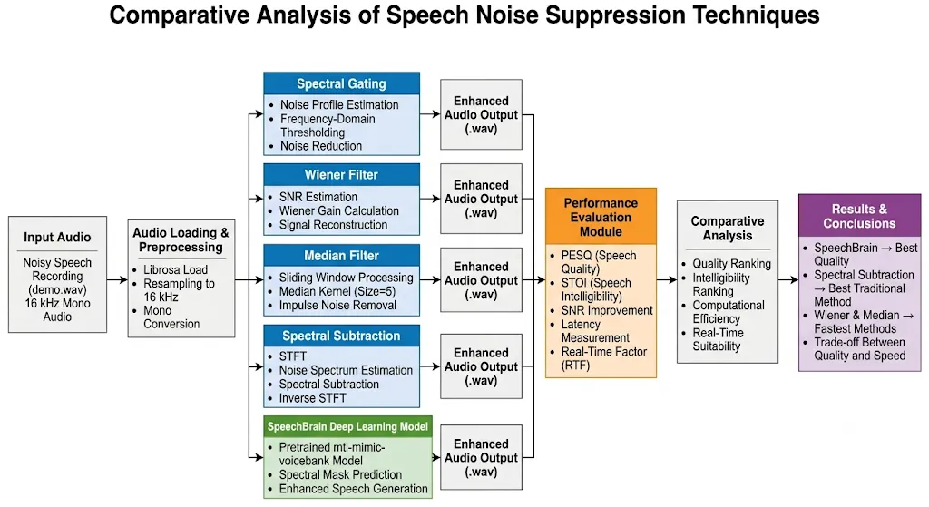
Comparative Analysis of Noise Suppression Models
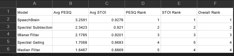
To evaluate the performance of different noise suppression techniques, a dataset of 100 noisy speech recordings was used. Each audio file was processed using all five models: SpeechBrain, Spectral Subtraction, Wiener Filter, Spectral Gating, and Median Filter. The enhanced outputs were then evaluated using PESQ (Perceptual Evaluation of Speech Quality) and STOI (Short-Time Objective Intelligibility), two widely used metrics for assessing speech quality and intelligibility.
The experimental results indicate that SpeechBrain achieved the best overall performance, obtaining the highest average PESQ score of 3.2591 and the highest average STOI score of 0.9278. This demonstrates the effectiveness of deep learning-based approaches in preserving speech characteristics while suppressing background noise. SpeechBrain consistently produced clearer and more natural-sounding speech across the majority of the 100 test recordings.
Among the traditional signal-processing methods, Spectral Subtraction delivered the strongest performance with an average PESQ score of 2.3423 and an average STOI score of 0.9210, making it the best non-deep-learning technique in this study. Wiener Filter closely followed, achieving good speech intelligibility while maintaining low computational complexity. These results suggest that both methods are suitable choices when computational resources are limited.
Spectral Gating and Median Filter showed comparatively lower performance. While these techniques were effective in reducing certain types of noise, they were less successful in preserving overall speech quality across the diverse set of recordings. Nevertheless, their low computational requirements make them attractive for applications where speed and simplicity are more important than achieving the highest possible enhancement quality.
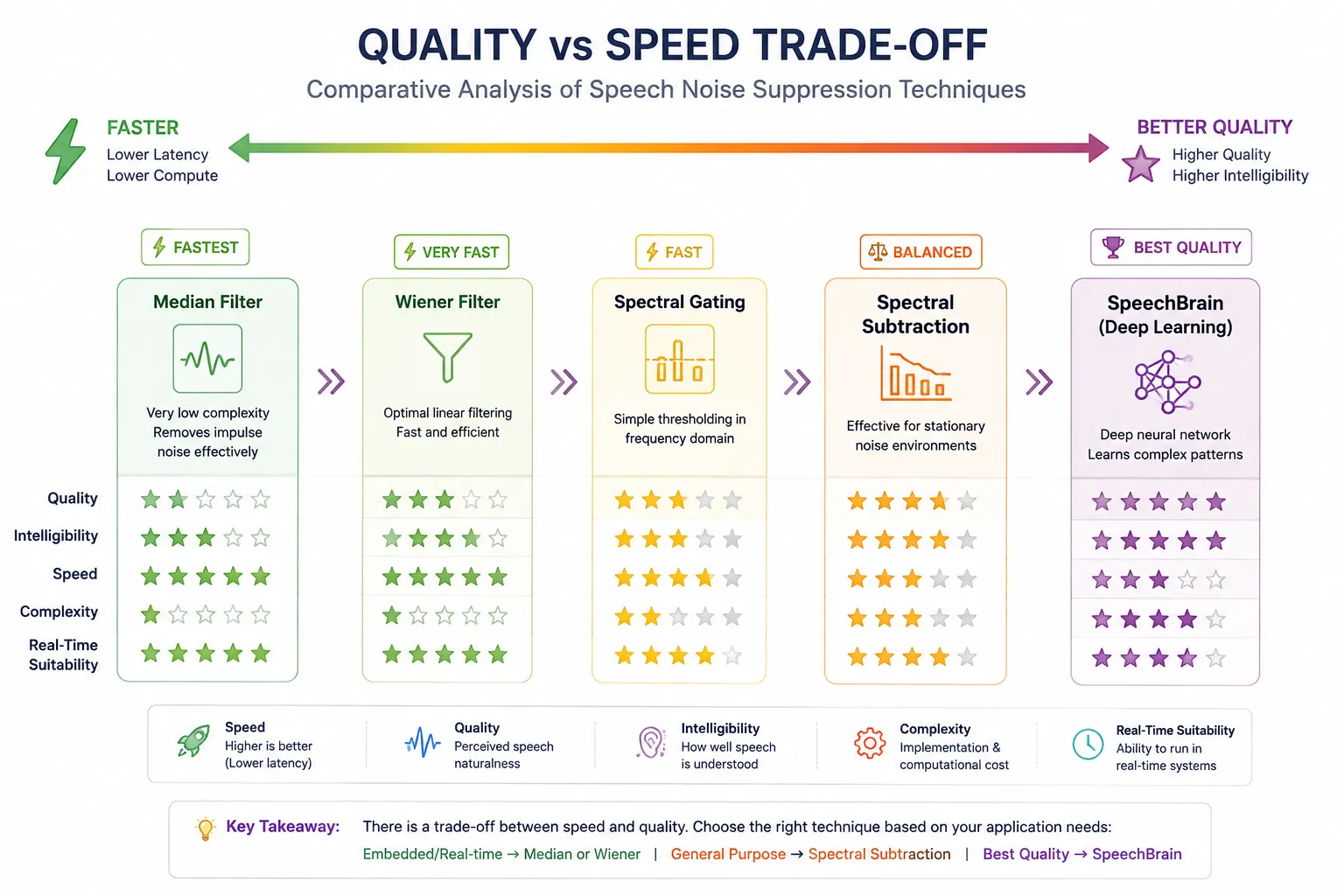
Based on the average PESQ and STOI scores obtained from the 100-audio-file dataset, the overall ranking of the models was: SpeechBrain > Spectral Subtraction > Wiener Filter > Spectral Gating ≈ Median Filter. The results highlight the trade-off between enhancement quality and computational efficiency, with SpeechBrain offering superior speech quality and intelligibility, while traditional methods provide faster and more resource-efficient processing.
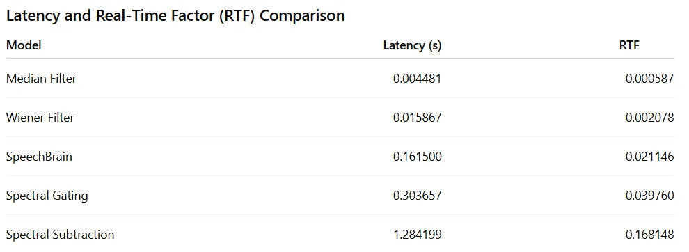
The latency benchmarking was performed on a 7.64-second audio sample to evaluate the computational efficiency of each noise suppression technique. The results show that Median Filter achieved the lowest latency (0.004481 s) and the smallest RTF (0.000587), making it the fastest method among all evaluated models. Wiener Filter also demonstrated excellent computational efficiency with a latency of only 0.015867 s, making it suitable for real-time and resource-constrained applications.
Among the more advanced methods, SpeechBrain achieved a latency of 0.161500 s and an RTF of 0.021146, indicating that it can process audio significantly faster than real time while providing superior speech quality. Spectral Gating required slightly more processing time (0.303657 s) but still maintained an RTF well below 1, making it suitable for practical deployment. Spectral Subtraction exhibited the highest latency (1.284199 s) among the tested methods due to the additional frequency-domain processing involved in STFT and inverse STFT operations.
Since all models achieved an RTF less than 1, every technique is capable of processing audio faster than real time. The results highlight the trade-off between computational efficiency and enhancement quality: traditional filters such as Median and Wiener are extremely fast, while SpeechBrain offers significantly better speech quality at the cost of moderately higher computation. Overall, SpeechBrain provides the best balance between enhancement performance and processing speed for modern speech enhancement applications.
Note: The latency and RTF values shown above were measured using a single audio file of duration 7.64 seconds. These values may vary depending on factors such as audio length, sampling rate, hardware configuration (CPU/GPU), noise complexity, and implementation details. Therefore, the reported results should be considered representative of the current experimental setup rather than absolute performance measurements.
Audio Output Summary
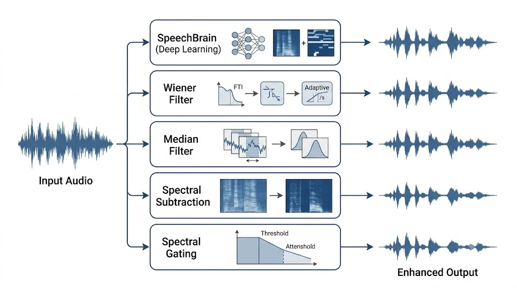
The five output files represent what each method sounds like after processing the same noisy input:
| File | Method |
|---|---|
| demo.wav | Original Noisy input |
| spectral_gating_demo.wav | Spectral Gating output |
| wiener_demo.wav | Wiener Filter output |
| median_demo.wav | Median Filter output |
| spectral_subtraction_demo.wav | Spectral Subtraction output |
| speechbrain_demo.wav | SpeechBrain output |
SpeechBrain produced the cleanest output — because it was trained specifically to learn what real speech sounds like versus what noise looks like. It can handle time-varying, non-stationary noise that completely confuses rule-based methods.
Wiener Filter and Median Filter were the fastest — they’re essentially single-pass array operations. If you’re building something that runs on a microcontroller or a Raspberry Pi, these are your friends. The trade-off is that they’re limited in how much noise they can actually remove.
Spectral Subtraction and Spectral Gating sit in the middle — they do a reasonable job on steady noise (like a room tone or fan) and are fast enough for most offline applications. But they both suffer from musical noise artifacts, where the residual noise sounds like a faint, flickering tone.
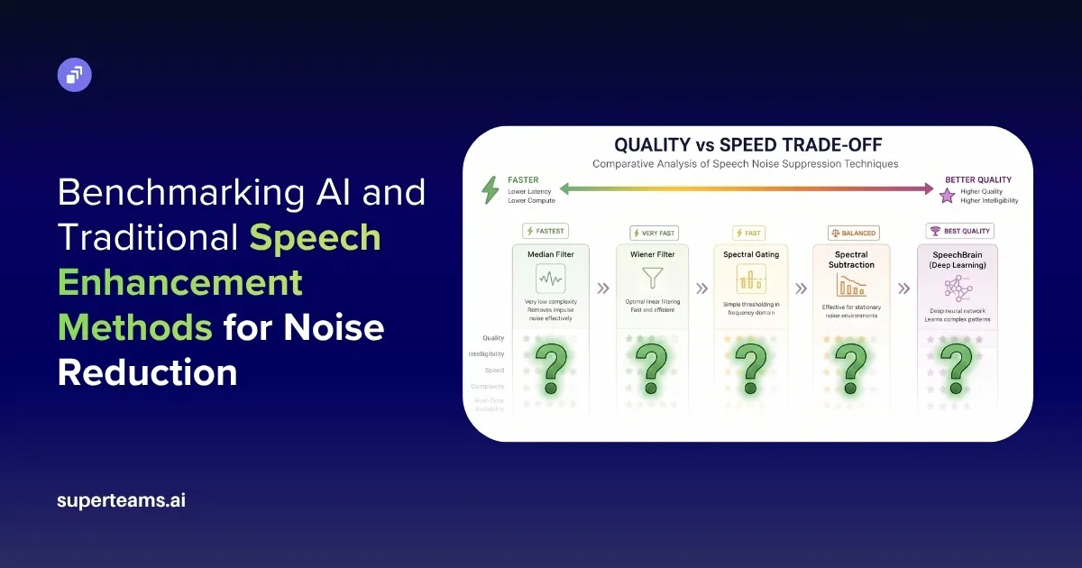
The fundamental trade-off is quality vs. speed:
- More compute = better quality (SpeechBrain)
- Less compute = faster, but noisier output (Wiener, Median)
Traditional methods make assumptions (noise is stationary, noise is Gaussian). Real noise breaks those assumptions constantly. Deep learning methods don’t assume — they learn. That’s why they win on quality, but at a cost.
To Summarize
While the current study demonstrates the effectiveness of both traditional and deep learning-based noise suppression techniques, there is significant scope for further improvement. Future work can focus on optimizing deep learning models for real-time deployment, exploring hybrid approaches that combine traditional filtering with neural networks, and evaluating lightweight speech enhancement models for edge devices. Additionally, recent transformer-based architectures have shown promising results in challenging noise environments and could be investigated to achieve even better speech quality and intelligibility.
In this study, five speech enhancement techniques were evaluated using self-recorded noisy speech samples and compared based on speech quality, intelligibility, latency, and real-time performance. The results demonstrated that SpeechBrain achieved the best overall enhancement quality, while traditional methods such as Wiener Filter and Median Filter provided faster processing with lower computational requirements. This comparison highlights the trade-off between performance and efficiency, showing that the optimal choice depends on the application requirements. Overall, deep learning-based approaches show great potential for delivering high-quality speech enhancement in real-world noisy environments.
Colab Notebook
The complete source code and implementation details for this project are available in the Google Colab notebook below:
https://colab.research.google.com/drive/1xZt3yb5-88JnjTFQT9Or0I89Mcejheuf
At Superteams, we help you build AI agents customized to your business needs. To learn more, speak to us.


-Feature-Image.CjBFdO7y_Z1JlSjK.webp)