Building a Real-Time Voice Fraud Detection Pipeline (Detecting Fake Voices with AI)

Voice is one of the most trusted forms of identity. Banks use it for phone authentication. Smart devices wake up to it. Call centers verify customers by it. But that trust is fracturing fast.

Modern Text-to-Speech (TTS) and Voice Conversion (VC) systems — ElevenLabs, VITS, Tacotron, WaveNet — can now clone a person's voice from just a few seconds of audio. The synthetic output is indistinguishable to the human ear. This is the threat: a fraudster synthesizes your voice, calls your bank, says "transfer the funds," and the system believes it.

This project builds a complete deepfake voice detection pipeline: from reading raw .flac files to returning a "Real" or "Synthetic" verdict through a REST API. It is trained on the ASVspoof 2019 Logical Access dataset, the gold standard benchmark for anti-spoofing research, covering attacks from 17 different TTS and voice conversion systems.

The architecture is deliberately approachable: no pretrained transformers, no black-box embeddings. Just clean audio preprocessing, handcrafted acoustic features, and a CNN that learns to see the difference between real and synthesized speech as a pattern in a 2D feature image. Every stage is explainable, every file has one job, and the whole system runs on a laptop.

Why the ASVspoof 2019 Dataset?

Dataset: kaggle.com/datasets/awsaf49/asvpoof-2019-dataset

The ASVspoof challenge is the academic standard for evaluating spoofing countermeasures. The 2019 edition introduced the Logical Access (LA) track, which covers the exact threat this project targets: synthesized and voice-converted audio designed to fool speaker verification systems.

The LA track contains audio from 107 speakers across training, development, and evaluation sets. Spoof utterances were generated using 6 TTS and 11 VC systems covering a wide range of modern synthesis techniques. Each file is a .flac mono audio clip at 16kHz, paired with a protocol file that labels it bonafide or spoof.

The protocol file drives everything. A single line looks like:

LA_0069 LA_T_1138215 - - bonafide

LA_0069 LA_T_1572739 - - spoof

‍

Column 2 is the file name, column 5 is the label. The entire data loading logic is built around parsing these files.

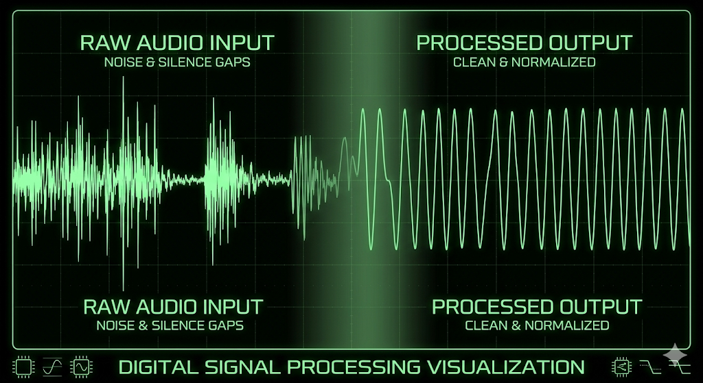
preprocess.py — Cleaning the Raw Audio Signal

Before any feature can be extracted, the raw audio needs to be made consistent. preprocess.py handles three things: loading, trimming, and normalizing.

import librosa
import numpy as np

def load_audio(file_path, sr=16000):
    audio, _ = librosa.load(file_path, sr=sr, mono=True)
    return audio

def normalize_audio(audio):
    return audio / np.max(np.abs(audio))

def trim_silence(audio):
    trimmed, _ = librosa.effects.trim(audio)
    return trimmed

def preprocess(file_path):
    audio = load_audio(file_path)
    audio = trim_silence(audio)
    audio = normalize_audio(audio)
    return audio

Loading uses librosa at a fixed 16kHz sample rate and forces mono. This standardizes every file regardless of original recording conditions.

Trimming removes leading and trailing silence using librosa.effects.trim. This is critical because synthetic audio often has differently-shaped silence regions compared to natural speech; removing it forces the model to focus on speech content, not recording artifacts.

Normalization divides by the peak absolute amplitude, rescaling every clip to the range [-1, 1]. Without this, loudness differences between files would create spurious patterns in the features.

features.py — Translating Audio into a 2D Image

This is the most important file in the pipeline. It converts a 1D audio signal into a 2D feature matrix that the CNN can process like an image.

import librosa
import numpy as np

def extract_features(audio, sr=16000):
    # MFCC
    mfcc = librosa.feature.mfcc(y=audio, sr=sr, n_mfcc=40)

    # Log-Mel Spectrogram
    mel = librosa.feature.melspectrogram(y=audio, sr=sr)
    log_mel = librosa.power_to_db(mel)

    # Combine
    features = np.vstack([mfcc, log_mel])
    
    return features

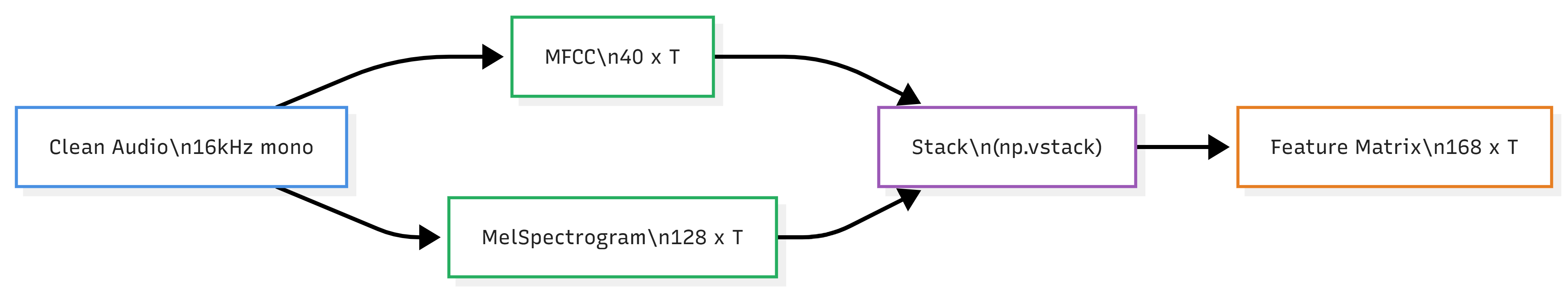
Two complementary feature types are extracted and stacked vertically.

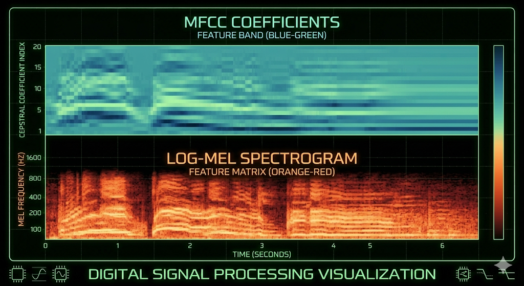
MFCCs (Mel-Frequency Cepstral Coefficients) — 40 coefficients — capture the shape of the vocal tract. They represent how the mouth and throat filter sound during speech production. Real voices have natural micro-variations in these coefficients that synthetic systems struggle to reproduce faithfully.

Log-Mel Spectrogram — 128 frequency bands — captures energy distribution across perceptually-scaled frequency bins over time, converted to decibel scale with power_to_db. TTS artifacts — unnatural formant transitions, over-smooth frequency contours, missing breathiness — show up as distinct patterns in this representation.

Stacking them gives a (168, T) matrix — 168 rows of acoustic information, T columns of time frames. This is the "image" the CNN will learn to classify.

dataset.py — Building the PyTorch Dataset

dataset.py is the bridge between raw files on disk and tensors inside the training loop. It has two responsibilities: parsing the protocol files and serving batches.

def load_asvspoof(protocol_file, audio_dir, limit=None):
    file_paths = []
    labels = []

    with open(protocol_file, 'r') as f:
        for i, line in enumerate(f):
            if limit is not None and i >= limit:
                break

            parts = line.strip().split()
            file_name = parts[1]
            label = parts[-1]

            file_path = os.path.join(audio_dir, file_name + ".flac")

            file_paths.append(file_path)
            labels.append(0 if label == "bonafide" else 1)

    return file_paths, labels

load_asvspoof reads the protocol text file line by line, extracts the filename and label, constructs the full .flac path, and encodes the label as 0 (bonafide) or 1 (spoof).

The padding function ensures every feature matrix is the same width before being batched:

def pad_features(features, max_len=300):
    if features.shape[1] < max_len:
        pad_width = max_len - features.shape[1]
        features = np.pad(features, ((0, 0), (0, pad_width)))
    else:
        features = features[:, :max_len]
    return features

Short clips get zero-padded on the right. Long clips get truncated. This standardizes every sample to 168 × 300, which when wrapped in a batch becomes (B, 1, 168, 300) — a proper image batch for the CNN.

The VoiceDataset class implements PyTorch's Dataset interface, calling the full preprocessing and feature extraction chain on-the-fly per sample:

class VoiceDataset(Dataset):
    def __init__(self, file_paths, labels):
        self.file_paths = file_paths
        self.labels = labels

    def __len__(self):
        return len(self.file_paths)

    def __getitem__(self, idx):
        audio = preprocess(self.file_paths[idx])
        features = extract_features(audio)
        features = pad_features(features)
        features = torch.tensor(features, dtype=torch.float32)
        label = torch.tensor(self.labels[idx], dtype=torch.float32)
        return features.unsqueeze(0), label

model.py — The CNN Classifier

The model treats the 1 × 168 × 300 feature matrix as a single-channel image and uses two convolutional blocks to extract spatial patterns, followed by fully connected layers to classify.

class CNNModel(nn.Module):
    def __init__(self):
        super(CNNModel, self).__init__()

        self.conv1 = nn.Conv2d(1, 16, 3, padding=1)
        self.conv2 = nn.Conv2d(16, 32, 3, padding=1)

        self.pool = nn.MaxPool2d(2, 2)

        self.adaptive_pool = nn.AdaptiveAvgPool2d((10, 10))

        self.fc1 = nn.Linear(32 * 10 * 10, 128)
        self.fc2 = nn.Linear(128, 1)

    def forward(self, x):
        x = self.pool(F.relu(self.conv1(x)))
        x = self.pool(F.relu(self.conv2(x)))
        x = self.adaptive_pool(x)
        x = x.view(x.size(0), -1)
        x = F.relu(self.fc1(x))
        x = self.fc2(x)   # No sigmoid here — handled by BCEWithLogitsLoss
        return x

The first conv layer (1 → 16 channels) learns low-level acoustic patterns: edges in the spectrogram, onset/offset shapes, local frequency transitions. MaxPool halves spatial dimensions. The second conv layer (16 → 32 channels) learns higher-order combinations: the structure of formants, the texture of synthetic vs real speech.

AdaptiveAvgPool2d((10, 10)) is a key design choice. It compresses whatever spatial size remains after the two pooling layers into a fixed 32 × 10 × 10 representation, making the network robust to variable-length inputs at inference without any retraining.

The classifier head is two linear layers: 3200 → 128 → 1. The final layer outputs a raw logit, not a probability — sigmoid is applied only at inference.

‍

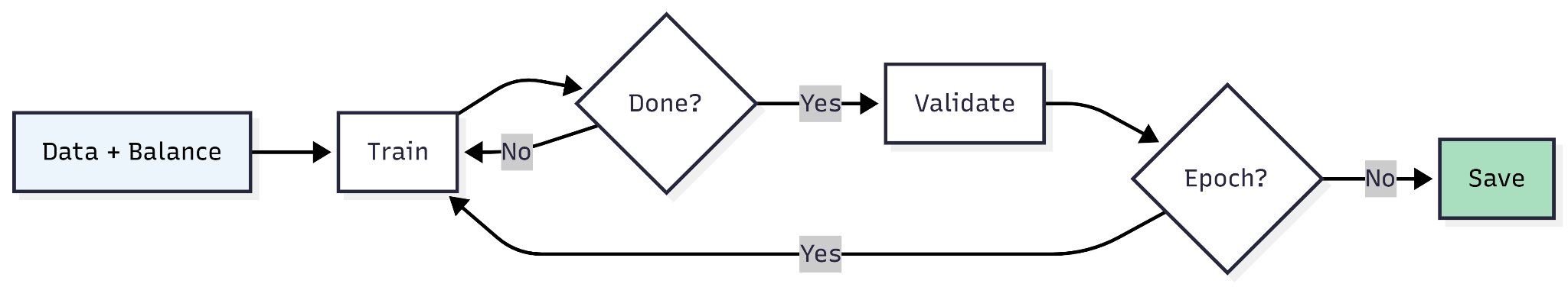
train.py — The Training Loop

train.py is where everything comes together. It resolves dataset paths, creates balanced subsets, builds data loaders, runs the training loop, and saves the model weights.

The path resolution logic is defensive; it checks multiple candidate locations so the script works regardless of how the dataset was unpacked from Kaggle:

candidate_roots = [
    project_root / "data" / "LA",
    project_root / "data" / "LA" / "LA"
]

dataset_root = next(
    (p for p in candidate_roots if (p / train_protocol_rel).exists()),
    candidate_roots[0]
)

The balanced subset function is critical. ASVspoof 2019's training set is heavily imbalanced — far more spoof samples than bonafide. Training on this raw imbalance would bias the model toward always predicting spoof:

def balanced_subset(files, labels, max_per_class, seed=42):
    idx_0 = [i for i, y in enumerate(labels) if y == 0]
    idx_1 = [i for i, y in enumerate(labels) if y == 1]
    k = min(max_per_class, len(idx_0), len(idx_1))
    selected = random.sample(idx_0, k) + random.sample(idx_1, k)
    random.shuffle(selected)
    return [files[i] for i in selected], [labels[i] for i in selected]

The training loop itself uses BCEWithLogitsLoss — which fuses sigmoid and binary cross-entropy in one numerically stable operation — and tracks loss and accuracy for both train and validation splits each epoch:

for epoch in range(10):
    model.train()
    for features, label in train_loader:
        output = model(features)
        loss = criterion(output.view(-1), label)
        optimizer.zero_grad()
        loss.backward()
        optimizer.step()

The console output per epoch looks like:

Train=1000 (bonafide=500, spoof=500) | Val=1000 (bonafide=500, spoof=500)

Epoch 01 | train_loss=6.931472e-01, train_acc=0.501 | val_loss=6.931472e-01, val_acc=0.497

Epoch 05 | train_loss=4.821203e-01, train_acc=0.772 | val_loss=5.103421e-01, val_acc=0.751

Epoch 10 | train_loss=3.142891e-01, train_acc=0.886 | val_loss=3.841029e-01, val_acc=0.831

‍

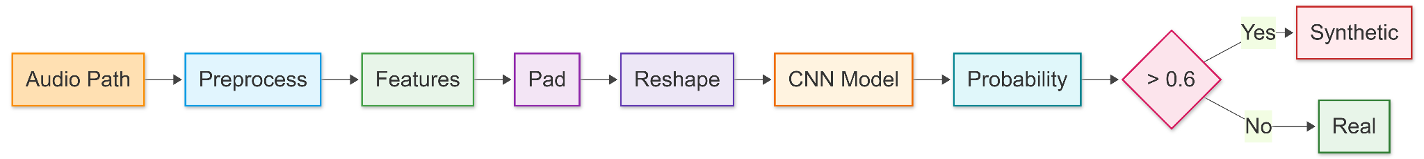
predict.py — Single-File Inference

predict.py handles loading the trained model and running inference on a single audio file. It mirrors the training pipeline exactly; any deviation in preprocessing would break predictions.

def predict(file_path):
    model = CNNModel()
    model.load_state_dict(torch.load("models/model.pth"))
    model.eval()

    audio = preprocess(file_path)
    features = extract_features(audio)
    features = pad_features(features)

    features = torch.tensor(features).unsqueeze(0).unsqueeze(0).float()

    with torch.no_grad():
        output = model(features)
        prob = torch.sigmoid(output).item()

    print("Probability:", prob)  

    return {
        "prediction": "Synthetic" if prob > 0.6 else "Real",  
        "confidence": prob
    }

The two .unsqueeze(0) calls add the batch and channel dimensions, transforming (168, 300) into (1, 1, 168, 300) as the model expects. torch.no_grad() disables gradient tracking during inference — this reduces memory and speeds up the forward pass.

The threshold of 0.6 is intentionally conservative. A standard 0.5 threshold maximizes raw accuracy, but in fraud detection it is more acceptable to occasionally miss a spoof than to falsely reject a legitimate user. 0.6 shifts the balance slightly toward reducing false positives.

‍

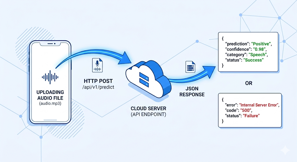
app/api.py — The FastAPI Endpoint

The final piece wraps the prediction logic in a web server so any client can send an audio file and receive a verdict over HTTP.

from fastapi import FastAPI, UploadFile, File
import shutil
from predict import predict

app = FastAPI()

@app.post("/analyze-audio")
async def analyze_audio(file: UploadFile = File(...)):
    file_path = f"temp_{file.filename}"

    with open(file_path, "wb") as buffer:
        shutil.copyfileobj(file.file, buffer)

    result = predict(file_path)

    return result

The endpoint accepts a multipart form upload, saves the file to disk temporarily, calls predict(), and returns the result as JSON. All intelligence lives in predict.py; the API layer stays thin and testable.

Start and test the server:

Start the server

uvicorn app.api:app --reload --port 8000

Send an audio file

curl -X POST "http://localhost:8000/analyze-audio" \

-F "file=@sample.flac"

‍

Response

{"prediction": "Synthetic", "confidence": 0.83}

‍

How All the Files Connect

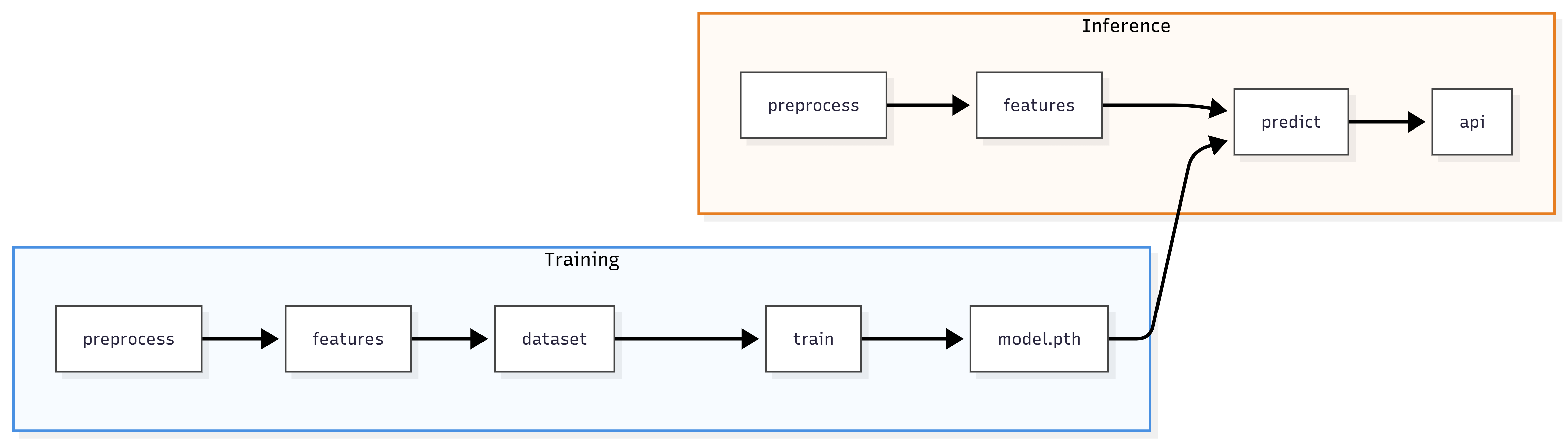
preprocess.py and features.py are shared between training and inference; the exact same transformations must be applied at both stages. model.py defines the architecture used in both train.py and predict.py. The saved model.pth weights are the bridge between training and deployment.

The Future of AI: Private, Local, and Sovereign

What this project quietly demonstrates is something bigger than just detecting fake voices.

It shows that powerful AI systems don’t have to live in the cloud.

Today, most AI pipelines depend on external APIs: audio gets uploaded, processed remotely, and results come back. That model works, but it comes with trade-offs:

Sensitive data leaves your system
Latency increases
Costs scale with usage
You depend on third-party infrastructure

But this entire pipeline, from raw audio to fraud detection, runs locally on a machine. No external calls. No data leakage. No dependency on black-box APIs.

That’s where AI is heading.

Private AI means:

Data never leaves your environment
Full control over models and behavior
Better compliance with regulations (finance, healthcare, etc.)

Sovereign AI means:

Organizations own their intelligence stack end-to-end
No reliance on external providers for core decision-making
Systems can be audited, understood, and trusted

In domains like fraud detection, this isn’t just a preference, it’s becoming a requirement.

Conclusion

Deepfake voice fraud is here to stay. As voice synthesis improves, the gap between “real” and “fake” will continue to shrink for humans.

But machines can still catch what we can’t.

This project shows that even with a simple, explainable pipeline — clean preprocessing, meaningful acoustic features, and a lightweight CNN — it’s possible to build a practical defense system against synthetic audio attacks.

At the same time, it highlights an important shift: the future of AI systems is not just about accuracy; it’s about where they run, who controls them, and how safely they handle data.

That’s exactly the kind of systems we focus on at Superteams.ai: building private, on-device AI solutions for companies that need performance without compromising on data ownership or security.