Building a Real-Time Sensor Anomaly Detection System with Qdrant Edge

Detecting Unknown Anomalies in Data

We wanted to explore whether anomaly detection could work without the usual constraints — no labelled data, no heavy cloud setup, and no dependency on pre-defined failure patterns. Most traditional approaches we came across either relied on historical failure labels (which aren’t always available) or required sending data to the cloud, introducing latency and complexity.

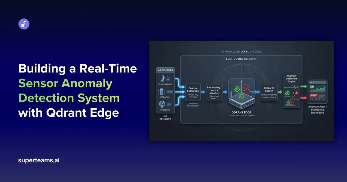
So we experimented with building a fully edge-based system that learns continuously from live data, adapts in real time, and detects anomalies within milliseconds — all without any prior training examples.

The Architecture at a Glance

Sensor Data (Temp, Humidity, Vibration)
          │
          ▼
  Feature Extraction (5 stats × 3 sensors = 15D vector)
          │
          ▼
  QdrantEdgeEngine  ←──── cosine similarity search
     (local shard)  ──────stores "normal" vectors
          │
          ▼
  AnomalyDetector
     ├── WARMUP PHASE      → learn the baseline
     ├── STABILIZING PHASE → observe without storing
     └── DETECTING PHASE   → Z-score anomaly flagging
          │
          ▼
  Streamlit Dashboard (real-time charts + alerts)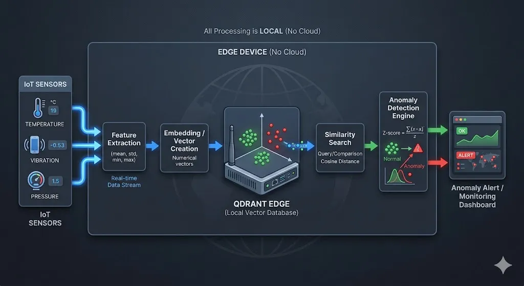

‍

Step 1 — Feature Engineering: From Raw Sensors to Vectors

Raw sensor readings are noisy and highly time-coupled. Instead of sending individual readings into the detector, we extract a 15-dimensional statistical feature vector from a sliding window of the last 10 readings.

For each of the 3 sensors (temperature, humidity, vibration), we compute 5 statistics: mean (average level), std (spread/volatility), min (floor of the window), max (ceiling), and delta (trend as last − first value). This is done in the main loop:

window_np = np.array(window)   # shape: (10, 3)
features  = []
for j in range(window_np.shape[1]):
    col = window_np[:, j]
    features.extend([
        col.mean(),
        col.std(),
        col.min(),
        col.max(),
        col[-1] - col[0]   # trend
    ])

vector = np.array(features)   # shape: (15,)

‍

The result is a compact 15-dimensional snapshot of recent sensor behaviour — not just instantaneous values.

Step 2 — Qdrant Edge: A Vector Database That Lives on Your Machine

We chose Qdrant Edge for this system because we wanted something that could give us the power of a full vector database without forcing us to run and manage a separate service. Since our goal was to keep everything lightweight and fast on the edge, the fact that it runs in-process and persists data locally made it a natural fit. It allowed us to keep the architecture simple while still achieving very low latency—something that’s critical for real-time anomaly detection.

We initially considered simpler approaches using Python lists or NumPy for similarity search, but it quickly became clear that scaling those efficiently would require a lot of extra work. With Qdrant Edge, we get optimized vector indexing, fast nearest-neighbor queries, and built-in persistence out of the box. That lets us focus on the anomaly detection logic itself rather than reinventing infrastructure, making it a practical and scalable choice for this system.

Qdrant is typically used as a cloud or containerised vector search engine. But Qdrant Edge is a lightweight embedded variant — it runs in-process, no server needed, and persists to a local directory.

Here's the entire storage engine:

class QdrantEdgeEngine:

    def __init__(self, fresh: bool = True):
        path = config.QDRANT_SHARD_PATH

        cfg = EdgeConfig(
            vectors={
                config.VECTOR_NAME: EdgeVectorParams(
                    size=config.VECTOR_SIZE,      # 15 dimensions
                    distance=Distance.Cosine,
                )
            }
        )

        if fresh and _shard_exists(path):
            shutil.rmtree(path)        # fresh session → wipe old data

        os.makedirs(path, exist_ok=True)
        self._shard = EdgeShard.create(path, cfg)
        self._count = 0
        self._id_counter = 0

    def store(self, vector: np.ndarray):
        """Persist a normal-behaviour vector to the shard."""
        self._id_counter += 1
        point = Point(
            id=self._id_counter,
            vector={config.VECTOR_NAME: vector.tolist()},
        )
        self._shard.update(UpdateOperation.upsert_points([point]))
        self._count += 1

    def search(self, vector: np.ndarray) -> float:
        """Return average cosine similarity against top-K stored vectors."""
        if self._count == 0:
            return 1.0                 # nothing stored yet → assume normal

        k = min(config.TOP_K_SEARCH, self._count)
        req = QueryRequest(
            query=Query.Nearest(query=vector.tolist(), using=config.VECTOR_NAME),
            limit=k,
        )
        results = self._shard.query(req)
        return float(np.mean([r.score for r in results]))

‍

Why cosine similarity? Because it measures direction, not magnitude. A vector that has the same pattern but different scale will still score close to 1.0 — which is what we want for sensor behaviour comparison.

Step 3 — The Anomaly Detector: Three-Phase Detection

The core intelligence lives in AnomalyDetector. It runs through three distinct phases:

Phase 1 — WARMUP (Steps 1–80)

During warmup, the system learns what "normal" looks like by storing incoming vectors — but only if they don't look like spikes:

if self.step <= config.WARMUP_STEPS:
    if len(self.history) >= 5:
        arr = np.array(self.history)
        mean, std = arr.mean(), max(arr.std(), 1e-6)
        is_spike = (similarity - mean) / std < config.ZSCORE_ANOMALY_THRESHOLD
    else:
        is_spike = False

    if not is_spike:
        self.engine.store(vector)   # only store clean normals

    self.history.append(similarity)
    return AnomalyResult(self.step, similarity, False, "WARMUP")

‍

This prevents the baseline from being "poisoned" by early anomalies. Smart training, not blind recording.

Phase 2 — STABILIZING (Steps 81–100)

The system watches without storing or flagging — giving the similarity score time to settle:

if self.step <= config.STABILIZATION_STEPS:
    self.history.append(similarity)
    return AnomalyResult(self.step, similarity, False, "STABILIZING")

Phase 3 — LIVE DETECTION (Step 100+)

Now the real work begins. The system computes a dynamic Z-score against a rolling window of recent similarity scores:

arr = np.array(self.history)
mean = arr.mean()
std  = max(arr.std(), 1e-6)

z_score   = (similarity - mean) / std
is_anomaly = z_score < config.ZSCORE_ANOMALY_THRESHOLD   # default: -2.5

# Safe learning: only update baseline with confidently normal vectors
if not is_anomaly and z_score > config.ZSCORE_LEARN_THRESHOLD:  # default: -1.0
    self.engine.store(vector)

self.history.append(similarity)
return AnomalyResult(self.step, similarity, is_anomaly, f"Z={z_score:.2f}")

The Z-score threshold of -2.5 means this: flag a reading only if its similarity drops more than 2.5 standard deviations below the recent mean. This dramatically reduces false positives compared to a fixed threshold.

Step 4 — Configuration: All Knobs in One Place

To make the system easier to tune and experiment with, we brought all the key parameters into a single configuration block so we could quickly adjust thresholds, window sizes, and search behavior without touching the core logic. While building this, we realized that anomaly detection is highly sensitive to these values, so having everything centralized helped us iterate faster, debug more effectively, and adapt the system to different sensor setups.

‍

This configuration essentially acts as a control panel for the pipeline—defining how the baseline evolves, when something is flagged as anomalous, and when the system is allowed to learn—while also making the overall design cleaner and more reproducible for anyone exploring the project.

QDRANT_SHARD_PATH = "qdrant_data"

VECTOR_NAME = "sensor_vector"
VECTOR_SIZE = 15          # 3 sensors × 5 statistical features

WARMUP_STEPS         = 80
STABILIZATION_STEPS  = 100   # must be > WARMUP_STEPS

ZSCORE_ANOMALY_THRESHOLD = -2.5  # flag if z-score drops below this
ZSCORE_LEARN_THRESHOLD   = -1.0  # only learn if z-score is above this

BASELINE_WINDOW = 50     # rolling window size for dynamic stats
TOP_K_SEARCH    = 5      # average similarity over top-5 nearest vectors

CHART_SIMILARITY_REF_LINE = 0.97  # visual reference only

Tuning these values lets you trade off sensitivity vs. false-positive rate without touching any detection logic.

Step 5 — The Streamlit Dashboard

The dashboard gives a real-time view of everything happening under the hood:

Key design choices:

Rolling 200-step chart — the window slides right-to-left so you always see the most recent data,
Warmup zone shading — green tint on the chart clearly shows the learning period.
Live feed — colour-coded: green for normal, orange for warmup, red for anomalies.
Anomaly log — persists all flagged events with their similarity score and sensor values.

Anomaly Injection for Testing

The data simulator injects two types of anomalies randomly (~5% chance each):

# Temperature spike + vibration spike
if np.random.rand() < 0.05:
    temperature += np.random.uniform(40, 80)   # +40–80°C
    vibration   += np.random.uniform(3, 8)     # ×100–400 normal
    is_injected  = True

# Humidity crash
if np.random.rand() < 0.05:
    humidity -= np.random.uniform(30, 60)      # −30–60%
    is_injected = True

These injections produce vectors that are geometrically distant from the stored normals — their cosine similarity drops sharply, triggering the Z-score detector.

Results: What Does Detection Look Like?

After warmup (~80 steps), the similarity score stabilises between 0.96–0.99 for normal sensor readings. When an anomaly is injected:

The feature vector shifts dramatically (temperature mean/max, vibration std all spike).
Cosine similarity to stored normals drops to 0.80–0.90.
Z-score falls below -2.5.
Alert is triggered and logged immediately.

The entire detection latency is < 5ms — purely local vector math with no network calls.

This approach works well because it learns “normal” behavior without needing labeled data, using a rolling similarity window that adapts to gradual changes in sensor patterns. It avoids contamination by only storing confidently normal readings, while the Z-score threshold (−2.5) provides a statistically sound way to detect anomalies based on actual data variability. Cosine similarity ensures that pattern shape matters more than magnitude, and with Qdrant Edge running locally, detection is extremely fast.

Overall, the system shows that effective anomaly detection doesn’t require heavy ML pipelines. By combining vector search, statistical scoring, and a phased learning approach, it can self-learn from scratch, adapt over time, and detect anomalies in real time—all while running efficiently on lightweight hardware.

If you’ve followed along, you’ve seen how anomaly detection can be done without labelled data or cloud dependency by learning “normal” directly from live data. The key idea is simple: use similarity to define normal behavior and flag deviations in real time. We’d encourage you to experiment with the parameters and adapt this approach to your own use cases like sensors, logs, or user activity.