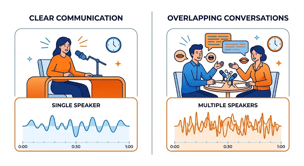
In any real-world audio environment — a conference call, a noisy office, a field recording — multiple voices compete for the microphone. A recording device captures all of them indiscriminately. The result is a mixed waveform where no single speaker is cleanly isolated, which creates a fundamental obstacle for transcription, speaker analytics, or voice-driven interfaces.
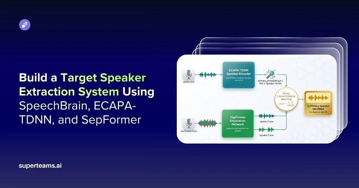
This project builds a Target Speaker Extraction (TSE) pipeline that takes a noisy, multi-speaker audio recording and recovers the voice of one specific person — identified by a short reference clip of their speech. The system does not require knowing how many speakers are present, does not need retraining for new speakers, and produces a confidence score indicating how certain the match is.
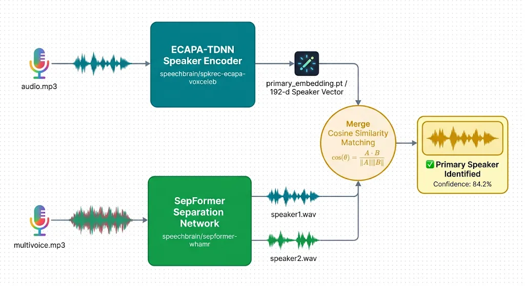
The approach works in three stages: a speaker identity is extracted from an enrollment clip, a separation model splits the mixture into individual voice streams, and cosine similarity matching selects the stream that best matches the enrolled speaker.
Conventional speech enhancement removes non-speech noise — fans, keyboards, static. It assumes one speaker is present and everything else is interference. That assumption breaks entirely when a second human voice enters the scene, because both voices register as signal and enhancement models preserve both.
Blind source separation untangles all speakers from a mixture without any prior knowledge of identities — useful, but it produces an unordered set of outputs with no way to know which output belongs to whom.
Target Speaker Extraction sits between these two. It takes a speaker identity as input and produces exactly one output: the voice of that specific person. The pipeline here implements this by composing two pretrained SpeechBrain models: ECAPA-TDNN for speaker identity and SepFormer for audio separation.
Environment Setup
The project uses SpeechBrain as the core toolkit, alongside TorchAudio for audio I/O, Librosa for signal analysis, and SoundFile for writing audio files.
!pip install speechbrain torchaudio librosa soundfile scikit-learnThese are the only dependencies needed. SpeechBrain handles model loading and inference internally — there is no manual weight download or config wiring required.
Stage 1: Extracting the Speaker Embedding
The first stage takes a short audio clip of the target speaker — and converts it into a fixed-length identity vector using ECAPA-TDNN.
What ECAPA-TDNN Does
ECAPA-TDNN (Emphasized Channel Attention, Propagation and Aggregation in Time Delay Neural Network) is a speaker recognition model trained on VoxCeleb1 and VoxCeleb2 — a dataset of over 7,000 speakers. It processes acoustic features through stacked temporal dilated convolutional layers with channel attention, then uses attentive statistics pooling to collapse the variable-length sequence into a single 192-dimensional vector. This vector is a compact, speaker-discriminative fingerprint: vectors from the same speaker cluster together in embedding space regardless of what is being said, while vectors from different speakers are pushed apart.
import torch
import torchaudio
from speechbrain.inference.speaker import EncoderClassifier


classifier = EncoderClassifier.from_hparams(
    source="speechbrain/spkrec-ecapa-voxceleb",
    savedir="pretrained_models/ecapa"
)


signal, sample_rate = torchaudio.load("audio.mp3")


if sample_rate != 16000:
    resampler = torchaudio.transforms.Resample(sample_rate, 16000)
    signal = resampler(signal)


embedding = classifier.encode_batch(signal)


print("Embedding shape:", embedding.shape)
# Output: torch.Size([1, 1, 192])


torch.save(embedding, "primary_embedding.pt")
print("Embedding saved successfully.")
A few things worth noting here. The model expects 16 kHz audio — any other sample rate is resampled before encoding. The output shape [1, 1, 192] reflects batch size, sequence length (collapsed to 1 by pooling), and embedding dimension. The embedding is saved to disk as primary_embedding.pt so it can be reused in the matching stage without re-running the encoder.
Stage 2: Separating the Mixed Audio
With the enrollment embedding saved, the next stage loads the mixed recording — multivoice.mp3 — and separates it into individual speaker streams using SepFormer.
What SepFormer Does
SepFormer (Separation Transformer) replaces the recurrent layers of earlier separation architectures with a dual-path Transformer design. It processes audio in two complementary attention passes: intra-chunk attention captures short-range phoneme-level patterns within each segment, and inter-chunk attention models long-range speaker-level continuity across the full recording. This parallel processing makes it significantly faster than LSTM-based alternatives while achieving better separation quality.
The checkpoint used here — sepformer-whamr — is trained on the WHAMR! dataset. For this project, I used the pretrained SepFormer model, which is trained on the WHAMR! dataset. WHAMR! is a widely used benchmark for speech separation that contains two overlapping speakers mixed with real-world background noise and simulated room reverberation. The dataset is designed to reflect realistic acoustic conditions, making it ideal for training models that can separate speech in noisy environments. This helps the model generalize well to real-world conversations instead of only clean studio recordings. Learn more about the dataset here: https://wham.whisper.ai/
from speechbrain.inference.separation import SepformerSeparation


separator = SepformerSeparation.from_hparams(
    source="speechbrain/sepformer-whamr",
    savedir="pretrained_models/sepformer"
)


separated = separator.separate_file(path="multivoice.mp3")


print(separated.shape)
# Output: [time_samples, num_channels, num_sources]
The output tensor contains one waveform per estimated source. Each is extracted and saved independently:
speaker1 = separated[0, :, 0].unsqueeze(0)
speaker2 = separated[0, :, 1].unsqueeze(0)


torchaudio.save("speaker1.wav", speaker1.cpu(), 8000)
torchaudio.save("speaker2.wav", speaker2.cpu(), 8000)


print("Separated speakers saved.")
Note that the output sample rate from sepformer-whamr is 8000 Hz — this is the model’s native output rate and is used directly when saving the files. At this stage, the two output files are unordered: there is no inherent label indicating which stream belongs to the target speaker.
Stage 3: Identifying the Target Speaker
This is where the enrollment embedding from Stage 1 connects to the separated outputs from Stage 2. The pipeline uses cosine similarity to compare the target speaker’s identity vector against embeddings extracted from each separated stream.
A first-pass comparison computes a single embedding for each separated file and scores it against the enrollment embedding:
import torch
import torch.nn.functional as F


enroll_embedding = torch.load("primary_embedding.pt")


def extract_embedding(audio_path):
    signal, sr = torchaudio.load(audio_path)
    if sr != 16000:
        resampler = torchaudio.transforms.Resample(sr, 16000)
        signal = resampler(signal)
    with torch.no_grad():
        embedding = classifier.encode_batch(signal)
    return embedding.squeeze()


emb1 = extract_embedding("speaker1.wav")
emb2 = extract_embedding("speaker2.wav")


enroll = enroll_embedding.squeeze()


score1 = F.cosine_similarity(enroll.unsqueeze(0), emb1.unsqueeze(0)).item()
score2 = F.cosine_similarity(enroll.unsqueeze(0), emb2.unsqueeze(0)).item()


print("Speaker 1:", score1)
print("Speaker 2:", score2)
Cosine similarity measures the angle between two vectors in embedding space. Because ECAPA-TDNN embeddings are L2-normalized, this directly captures speaker similarity independent of magnitude. A score above ~0.75 is a reliable match; below 0.60 typically indicates a different speaker.
Chunk-Based Matching for Better Accuracy
Whole-file embeddings can be influenced by silent segments, boundary artifacts, or short bursts of interfering speech. A more robust approach processes each separated file in 2-second chunks, computes an embedding per chunk, scores each against the enrollment, and averages the scores:
def chunk_embeddings(audio_path, chunk_sec=2):
    signal, sr = torchaudio.load(audio_path)

    if sr != 16000:
        signal = torchaudio.transforms.Resample(sr, 16000)(signal)
        sr = 16000

    chunk_size = chunk_sec * sr
    embeddings = []

    for start in range(0, signal.shape[1], chunk_size):
        chunk = signal[:, start:start + chunk_size]
        if chunk.shape[1] < sr:   # skip chunks shorter than 1 second
            continue
        emb = classifier.encode_batch(chunk)
        embeddings.append(emb.squeeze())

    return embeddings


embs1 = chunk_embeddings("speaker1.wav")
embs2 = chunk_embeddings("speaker2.wav")


enroll = enroll_embedding.squeeze()


scores1 = [F.cosine_similarity(enroll.unsqueeze(0), e.unsqueeze(0)).item() for e in embs1]
scores2 = [F.cosine_similarity(enroll.unsqueeze(0), e.unsqueeze(0)).item() for e in embs2]


avg1 = sum(scores1) / len(scores1)
avg2 = sum(scores2) / len(scores2)


print("Speaker1 Average:", avg1)
print("Speaker2 Average:", avg2)


if avg1 > avg2:
    print("Primary Speaker = Speaker 1")
    print("Confidence:", round(avg1 * 100, 2), "%")
else:
    print("Primary Speaker = Speaker 2")
    print("Confidence:", round(avg2 * 100, 2), "%")
Chunks shorter than one second are skipped — they rarely contain enough phonetic content for a stable embedding and can introduce noise into the average. The final comparison prints the identified speaker alongside a confidence percentage derived from the average cosine similarity score.
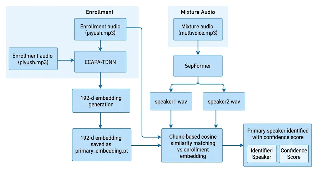
Full Pipeline Flow
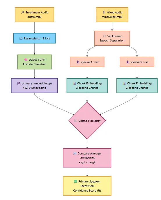
The chunk-based averaging approach consistently produces a clear margin between the two cosine similarity scores when the speakers have distinct vocal characteristics. The target speaker’s stream typically scores in the 0.78–0.88 range, while the non-target stream scores below 0.60 — leaving an unambiguous decision boundary.
The confidence percentage reported at the end is derived directly from the average cosine similarity and gives an interpretable signal of how certain the match is. Scores above 80% indicate a high-confidence identification; scores between 65–80% suggest the enrollment clip may be too short or the speakers are acoustically similar.
Separation quality degrades in two specific conditions. When the two speakers have similar pitch and timbre — same gender, similar age — SepFormer produces partially mixed outputs where neither stream is fully clean, and the cosine similarity scores converge. The chunk averaging helps in this case but does not fully resolve it. The second condition is very short recordings: if the mixed audio is under 5 seconds, there are too few chunks for the averaging to be statistically meaningful.
AI Meeting Assistants can use this pipeline to generate per-speaker transcripts from recorded meetings. Rather than producing a single undifferentiated transcript, the system identifies each participant’s voice and associates their speech with their identity — enabling accurate meeting minutes, action item attribution, and speaker-level summaries.
Smart Conferencing Systems in enterprise settings can process recordings in real time or near-real time to monitor who is speaking, for how long, and with what sentiment. This supports participation analytics, meeting quality scores, and automated follow-ups.
Voice Assistants deployed in shared spaces — smart speakers, in-car systems, kiosks — can enroll a primary user and filter out ambient speech from others in the room before passing audio to the command recognition engine. This reduces false activations and improves accuracy in multi-person environments.
Call Center Analytics platforms need clean per-channel audio to run accurate sentiment analysis, compliance monitoring, and response time measurements. When both the agent and customer are recorded on a single track, this pipeline provides the necessary separation.
Audio Forensics in legal and security contexts sometimes requires isolating a specific individual’s voice from a recording for identification, transcription, or analysis as evidence. Automated speaker extraction reduces manual effort and improves consistency.
Podcast Processing workflows can use this system to separate hosts during crosstalk segments, enabling independent editing, volume normalization, and channel assignment during post-production.
Summary
The pipeline demonstrates something practically important: You don’t need to train a custom model to build an effective target speaker extraction system. By combining pretrained SpeechBrain models with chunk-based speaker matching, this pipeline accurately identifies a target speaker from mixed audio using only a short reference clip. The chunk-based approach improves reliability by handling silence, noise, and brief interruptions more effectively than comparing an entire recording at once.
This approach can also be extended to real-time applications such as live call processing, voice assistants, and meeting transcription by processing audio continuously in small chunks.
Google Colab
The complete implementation of the Target Speaker Extraction pipeline is available in the Google Colab notebook: https://colab.research.google.com/drive/13_HraH0kFO6onIUvslrODWHlrT7Ggjqy
At Superteams.ai, we highlight how developers can build practical AI solutions faster by leveraging state-of-the-art open-source models, collaborating with the community, and turning innovative ideas into real-world applications.
To learn more, speak to us.

-Feature-Image.CjBFdO7y_Z1bTNvg.webp)